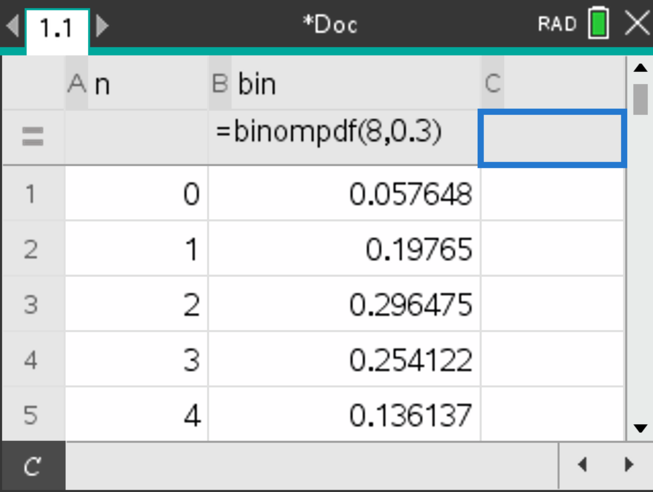
Consider \( X \sim \mathcal{B}(8, 0.3) \). Suppose you want to calculate \( P(X = 4) \)
 , select Probability > Distributions > Binomial Pdf
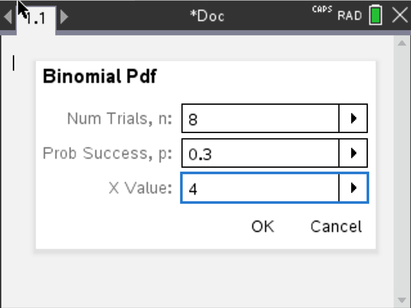
Press OK. The result should be 0.136 (rounded).
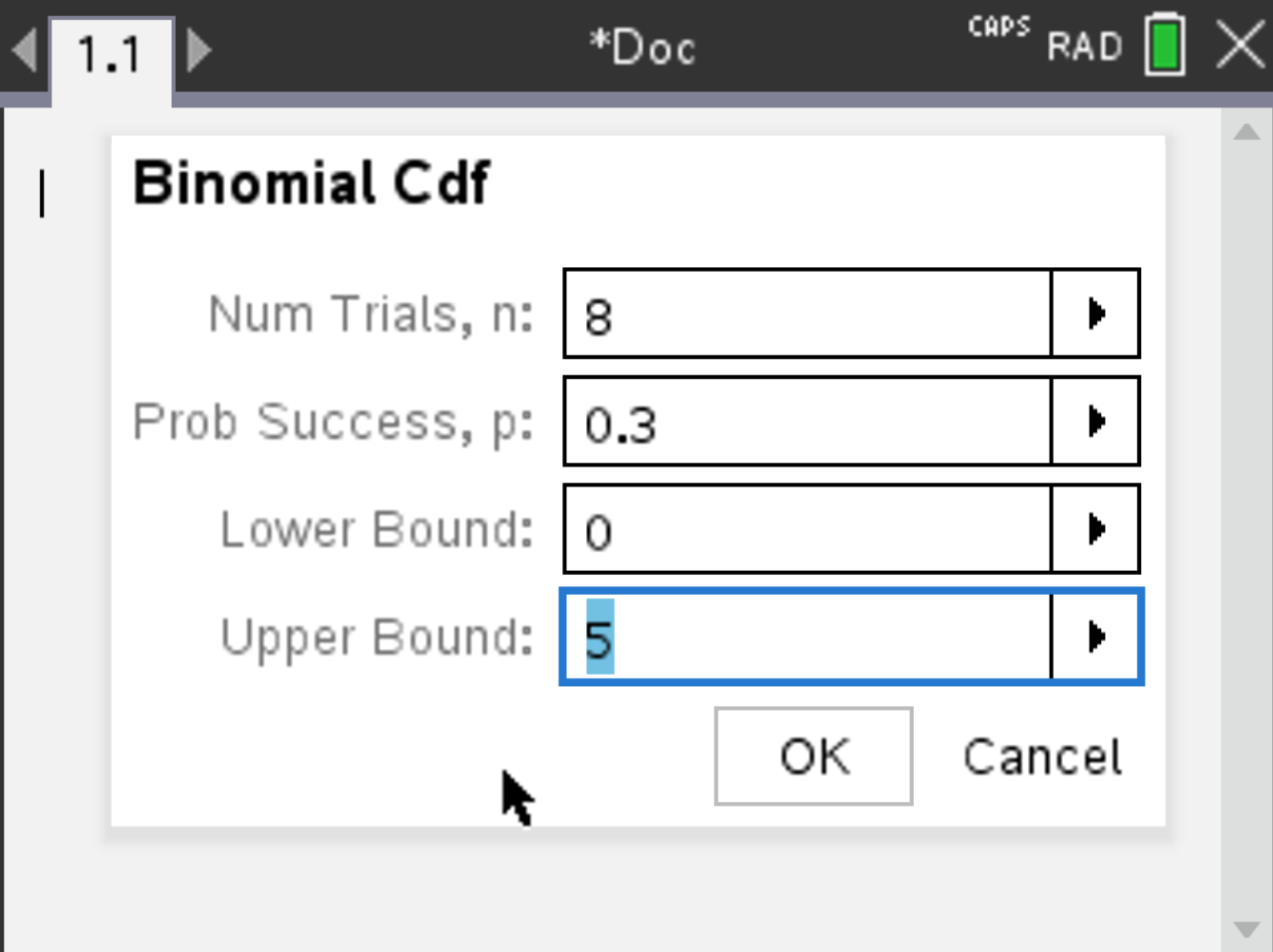
Consider \( X \sim \mathcal{B}(8, 0.3) \). Suppose you want to calculate \( P(X \leq 5) \)
, select Probability > Distributions > Binomial Cdf
 and the result is displayed. The result should be 0.988708.
NB: If you wanted to compute \( P(X < 5) \) instead, you would calculate \( P(X \leq 4) \) (since the binomial distribution is discrete).
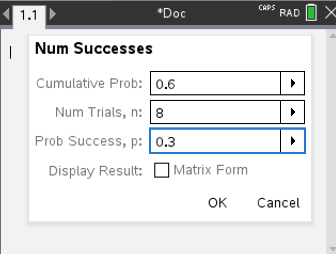
Consider \( X \sim \mathcal{B}(8, 0.3) \). Suppose you want to find the smallest x for which \( P(X \leq x) \geq 0.6 \).
, select Probability > Distributions > Inverse Binomial
and the result is displayed. The result should be 3.
Note that Binomial Cdf(8,0.3,3)=0.806, which is not 0.6. But since Binomial Cdf(8,0.3,2)=0.552 is smaller than 0.6, Inverse Binomial gives us 3 (even though 2 gives an area closer to 0.6, the calculator gives the first integer that gives an area bigger or equal to 0.6).

Pay attention to the discrepancy between the values!
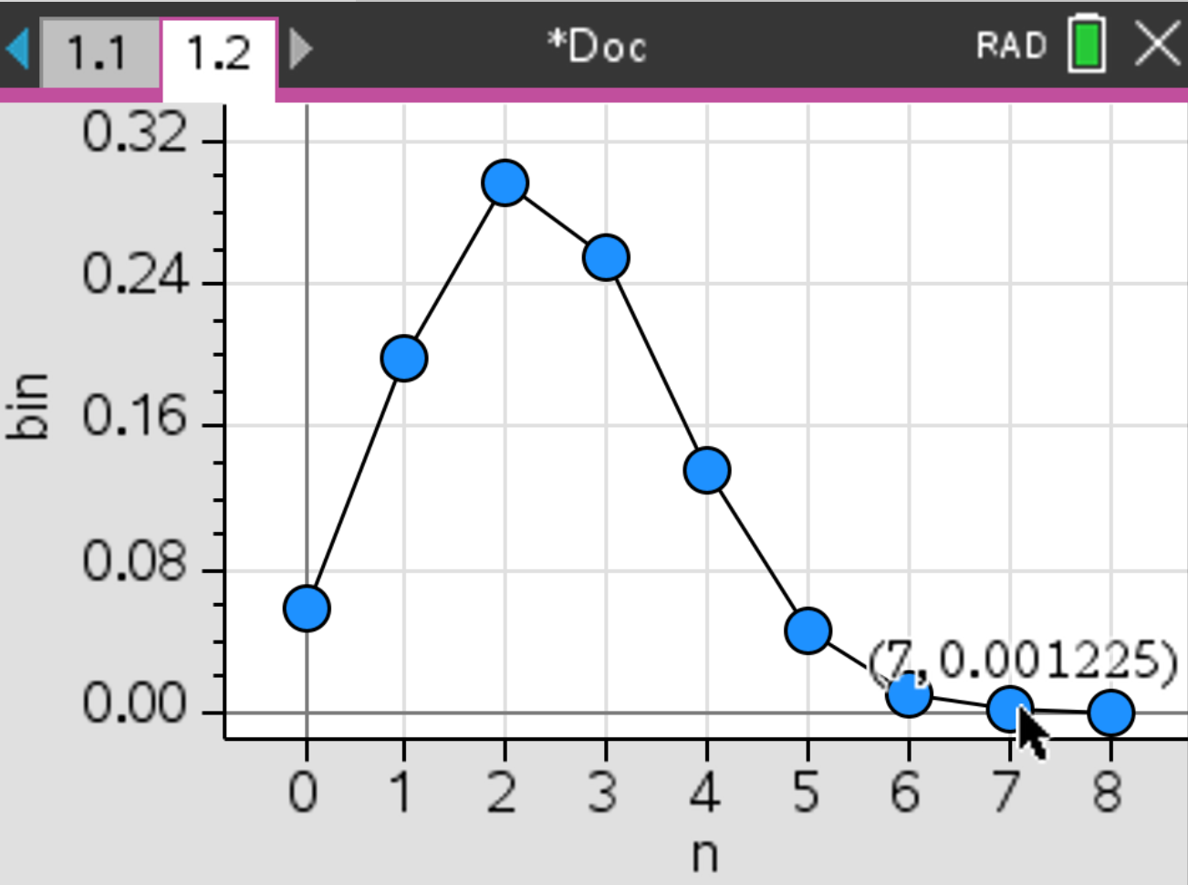
To plot a binomial distribution, we will create two lists, one being the possible amount of successful trials, and the other their probability, and then plot it.
and the probability of success for each number of trials is displayed.
 and
and  , select Add Data & Statistics.
, select Plot Properties > Connect Data Points. The following plot should be displayed:
, select Add Data & Statistics.
, select Plot Properties > Connect Data Points. The following plot should be displayed: